Digging Up a 17-Year-Old TIPE: SAW Touchscreens, Finite Differences, and a Half-Lost Simulation

The half I could find

For years I had a memory shaped like this: my prépa TIPE had been a CUDA project. Surface acoustic wave touchscreens, simulated on the GPU, parallelised, slightly cool. The memory turns out to be partly right and partly broken.

In April 2026 I went looking for the code. The OMV NAS I run at home still holds an image of the dying hard drive of my old Dell XPS desktop from prépa years. There is a directory under XPS/Antoine/Desktop/ dated 21 June 2009, with a complete simulation in C with SDL and OpenMP. There is also, separately, a single .cu file dated 19 June 2009: a 1.2 KB hello-world doing a 9-thread vector addition, sitting next to a downloaded paper by Balacey, Chatelard, Faure and Gilles on CUDA that I had clearly used as a reference at the time.

The CUDA version of the actual TIPE simulation, the one I remember writing and running on the lab GPU, is nowhere on the backup. It did exist. I am sure of that. It is gone now: lost between hard drives, lost in a directory that did not survive the format-and-reinstall cycle of an XPS that was already showing its age, lost in the way a 17-year-old project on a personal machine eventually loses its files. I cannot find it.

What I did find is the CPU twin: the same simulation, same physics, same input grid, written in plain C with SDL for the rendering and OpenMP for the parallelism. The CUDA work itself never touched a school machine: it ran on my own GPU at home, and on a friend’s freshly-built workstation (a serious new rig at the time, generous enough to lend out to a classmate working on a TIPE). Whether I wrote the CPU version as a baseline before the GPU port, or as a fallback for the moments I did not have access to either GPU, or simply because the development cycle was faster on the CPU, the records that would tell me are gone with the rest. What remains is one half of the project. It is the half that I am writing about here, because it is the half that came back to life.

What the TIPE was actually about

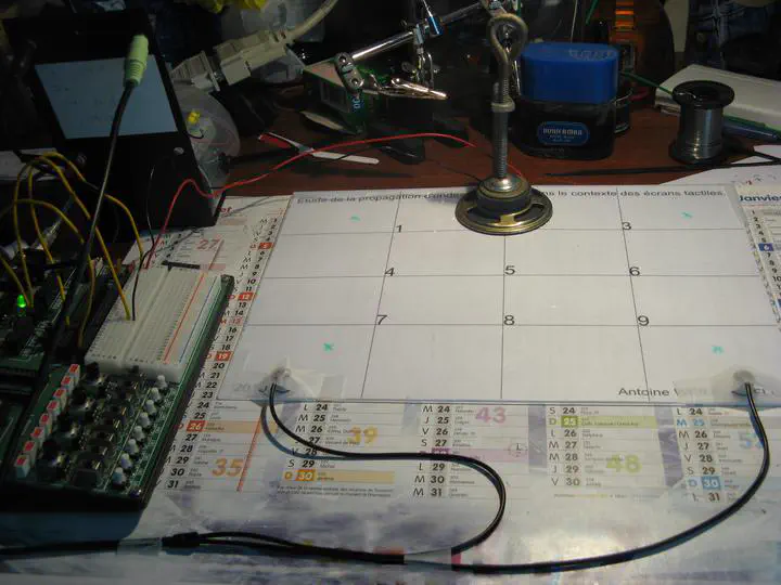
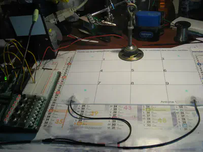
The full title is on the calendar in the photo above: Étude de la propagation d’ondes dans le contexte des écrans tactiles. The point of the project was to understand and partially reproduce a surface acoustic wave (SAW) touchscreen.

If you have used a public information kiosk, a casino slot machine, or some industrial control panels, you have probably touched a SAW screen without knowing it. Compared with the resistive and capacitive touchscreens we now have everywhere, SAW has some real advantages:

• Optical clarity is uncompromised. You are touching an unmodified piece of glass. There is no ITO layer in front of the display, so the brightness and contrast of the underlying screen are not degraded.
• It is robust against scratches. A scratch in a capacitive sensor changes the capacitance map. A scratch on the surface of a SAW glass plate barely affects how a wave propagates across it.
• It works through gloves. Capacitive needs a conductor. SAW only needs a finger (or anything else that absorbs vibration), so it works in winter, in the kitchen, in the operating room, and in factories.
• It works on bulletproof glass. The plate can be thick. This is why SAW has historically dominated public-facing kiosks, ATMs, and gaming machines.

In return, you give up two things: SAW is contact-only in its commercial form (no hover), and the spatial precision is lower than capacitive. You are not going to draw fine lines on a SAW screen. You will, however, click large buttons reliably for ten years in a humid arcade.

The PDF deck for the oral lays this out in the first three slides, and then the rest pivots to the question that interested the project: could we model a SAW screen well enough to understand why it works, and could we build one in a CPGE physics lab?

A note on context that does not appear in the deck. A friend, Élie, was working on his own wave simulation at the same time, in parallel and independently. His angle was the visual one: standing wave patterns, the Chladni-figure aesthetic, the same physics that lets you sprinkle salt on a vibrating plate and watch it organise itself onto the nodes. My angle was more practical: I wanted to push the touchscreen idea past what the commercial SAW screens of the time could do, and try to detect multi-touch and sliding gestures. Two fingers on the plate at once, each shifting the steady-state spectrum in its own way; or one finger moving across the plate, the spectrum continuously evolving as it goes. The lab demo on the deck stops at static single-touch, because nine out of nine on a 3 by 3 grid was what I got working robustly in time for the oral. The simulation itself was always being run with continuous excitation because that is what you need for multi-touch and motion: a steady sinusoidal source on the plate, the receivers humming along, and the spectrum reacting in real time to whatever you do on the surface.

The physics, in slightly less than a lecture

The wave equation on a plate is the classic 2D linear wave equation, with celerity c set by the material:

Δz = (1 / c²) · ∂²z / ∂t²

For an isotropic solid, c comes from the elastic properties: Young’s modulus E, Poisson’s ratio ν, and density ρ. The PDF works the example for plexiglas (acrylic glass: E = 2380 MPa, ν = 0.34, ρ = 1180 kg/m³), which gives a wave celerity of roughly 1500 m/s. Slow enough that a finite-difference simulation can run at a reasonable timestep, fast enough that a small plate has the modes you would expect from a real touchscreen.

You discretise the equation in the obvious way. Sample space at step dx and time at step dt, replace the Laplacian with its 5-point discrete cousin, and you get the explicit recurrence:

z(i, j, k+1) = 2·z(i, j, k) − z(i, j, k−1)
             + (c·Δt / Δx)² · [ z(i−1, j, k) + z(i+1, j, k)
                              + z(i, j−1, k) + z(i, j+1, k)
                              − 4·z(i, j, k) ]

That is the entire core of the simulation. Three time slices, two indices, one constant. Each cell only needs its four neighbours and its own previous values. This is embarrassingly parallel. It is also exactly the kind of problem where a 2009 dual-core CPU with OpenMP could already make real progress, which is precisely what the simulation does.

What the CPU simulation does

The code lives in five C files (main.c, simulation.c, simulation.h, events.c, events.h) plus a tiny utilitaire.h of macros, totalling under 30 KB of source. The features I cared about for the multi-touch angle were:

• A 501 by 501 grid of cells, drawn pixel-by-pixel into an SDL surface, with a square plate boundary (the simulation also supports a free edge and a disc-shaped plate, both more relevant to the standing-wave-pattern side of the project).
• Two independent oscillating sources, each with selectable waveform (sine, square, triangle, free-form), frequency, amplitude, and phase. You can drag them around the plate with the mouse. Two excitation points are useful when you start thinking about distinguishing more than one touch on the plate at once.
• Optional attenuation, a small velocity damping factor, so a run does not bounce forever.
• A perturbation tool: you click somewhere on the plate and the simulation imposes a local rest condition there, the way a finger touching a real plate would. This is the entire point of a SAW touchscreen, and the entire point of the simulation for me. Click to place a touch, watch the wavefield change, watch what the receivers see.
• State save and restore to text files, mapped to the O and I keys with the numeric keypad picking the slot. Useful for comparing the same configuration with and without a touch, which is the experiment in software form.
• OpenMP pragmas on the main update loops. The 2009 hardware was a dual-core CPU; the 2026 port runs comfortably on whatever you have.

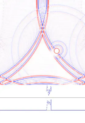
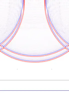
A clarification before the rest of this section reads strangely. The two clips above are the simulation in burst mode: a finite sine pulse, then silence, recorded as a clean impulse response. Burst mode is something I added to the program in 2026, purely because it makes a readable still and a readable loop. The actual 2009 work ran with continuous excitation: a sustained sinusoidal source, the receivers humming, the spectrum settling into a steady state, the perturbation tool moved around live. That is the regime where multi-touch and sliding gestures make sense, because both are defined by how the steady-state spectrum changes over time, not by an isolated impulse. A burst gives you a beautiful GIF. A continuous source gives you the actual interaction loop the project was about.

The visual quality is genuinely good. Standing in front of the running simulation in 2026, with the 5-point Laplacian doing its job at sixty frames per second, you can see why it works. Touch the plate, the nodes shift, the receivers see a different signal, the FFT sees a different spectrum, you read the position off the spectrum. The simulation is the explanation.

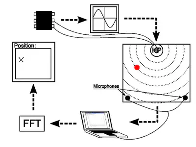
What I built in my room

The other half of the project, the half that justified the cas concret part of the deck, was an actual experimental rig. It is the photograph at the top of this post.

The hardware list is short and pleasant:

• A flat plate. The 3 by 3 calendar page in the photo is the test pattern; the actual plate I cannot reconstruct from memory with confidence.
• One speaker (HP in French schematics, haut-parleur), driven by a fixed-frequency signal generator. This is the SAW source.
• Two microphones stuck near two corners of the plate. With only two receivers, the position estimate has to come from spectral information rather than from time-of-flight triangulation.
• A laptop running Michael T Flanagan’s Java plotting library, used to FFT the recorded signal and read the dominant peaks.
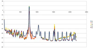
• A 3 by 3 test grid drawn on the test surface, marked 1 through 9. The deck shows the spectrum changing from position to position; the position estimation step uses those spectra to classify a new touch.

The result, as written on the conclusion slide, is:

• 9 out of 9 test positions correctly classified.
• Approximately 1 cm of spatial precision.
• A few classification errors that I attributed to the algorithm rather than the physics (“perfectible algorithm”).
• A surprising observation: out-of-contact detection seemed possible. Bringing a finger close to the plate, without touching, already changed the spectrum enough to be detectable. I did not push that hard at the time. In 2026, I look at that line in the slides and I want to go back and chase it.

Nine out of nine might not sound like much in isolation. Reach back into the constraints: a CPGE physics lab, two cheap microphones, a single fixed-frequency source, no calibration, and a Java FFT plot. As a proof of concept that you can build a working position-detection system with grocery-store hardware, it stood up.

The 2026 port: SDL 1.2 to SDL 2

The original code targets SDL 1.2. SDL 1.2 reached its end of life in 2012 and is no longer packaged on a modern distribution in any usable form. So the simulation as found on the NAS would not build, would not link, and would not run. Bringing it back was a small but real piece of work, done in April 2026 with Claude as a coding partner and tracked in the README of the recovered repository. The diff against the original copy is short:

• SDL_SetVideoMode is gone, replaced by SDL_CreateWindow plus SDL_GetWindowSurface.
• SDL_Flip(ecran) is gone, replaced by SDL_UpdateWindowSurface(fenetre).
• SDL_CreateThread grew a name argument in SDL 2 that did not exist in 1.2, so calls had to be updated.
• The keyboard API is the most invasive change. SDL 2 split keys into keycodes (which character was logically pressed) and scancodes (which physical key was pressed). The original code indexed an array by SDLK_* directly and assumed the values were contiguous up to SDLK_LAST + 1. They are not in SDL 2. The fix was to index by scancode instead, sized by SDL_NUM_SCANCODES, and to convert between the two with SDL_GetScancodeFromKey at the right boundary.
• A handful of keypad symbols were renamed (SDLK_KP0 to SDLK_KP_0, with the underscore).
• inline void calcul(...) had to become static inline for the linker to be happy under modern gcc, because pure C99 does not provide an external definition.

A few quirks of the original code survived the port. m_attenuation is declared int and used in two places that disagree on whether it is a boolean or a float multiplier. The SDLK_b key is bound to two different actions in the same key map and the first one in the linked list wins. Neither matters for the experiment. Both made me smile.

The result builds with MSYS2 mingw64 gcc 11.2.0 against SDL 2.30.10, runs on Windows with no installer, and produces the same visual output the original code did in 2009. The recovered repository, including the binary and the DLLs, lives on the home NAS. I have not put it on a public Git host yet, since it is not really my code to publish.

A coda from 2013

A few years later, around 2013, I met Charles Hudin and learned that he had been working on the exact inverse of what my TIPE was about. The paper that came out of that work, with my eventual PhD supervisor Vincent Hayward as a co-author, is Hudin, Lozada and Hayward, Localized Tactile Feedback on a Transparent Surface Through Time-Reversal Wave Focusing, IEEE Transactions on Haptics 8(2):188 to 198, 2015.

Same plate, same 2D wave equation, same 5-point Laplacian. The arrows pointing the other way. Where my TIPE used the waves arriving at edge sensors to figure out where a finger had been placed, Charles was using time-reversed signals re-emitted from edge transducers to focus a wavefront onto a chosen point on the plate, briefly enough and intensely enough to create a localized tactile sensation right under it. Detection on one side, generation on the other. The same simulation, played backwards in time.

It is the kind of connection you do not see coming. Once you do, a TIPE from 2009 stops feeling like a closed file and starts feeling like the first half of a longer thread.

What stuck

There is a pattern I keep noticing in my own technical history. The thing I remember from a project is rarely the result. It is the technique, or sometimes just a single image. From this TIPE the things I retained are the shape of the problem (a 5-point Laplacian on a regular grid is the canonical introduction to wave simulation, and it still is), the visual idea of nodal lines moving when you touch a plate, and the satisfaction of seeing nine out of nine on a confusion matrix. The CUDA work that I am sure I did, and whose source I cannot find, lives in my head as ambition rather than as code. That is also fine. Ambition that you remember well enough to describe is, in retrospect, more durable than code that you only remember as a filename.

Recovering the surviving half, file by file as I read through the 2009 source, was its own small archaeological pleasure: every variable name in the right French style, every API call obviously written by a CPGE student in a hurry.

There is a small irony in which half survived. The CUDA version was the impressive one in 2009, the one I would have wanted to show off, the one that would make a grader sit up. The CPU twin was, by comparison, the safe and obvious one. Seventeen years later, the safe and obvious one is the one that still runs. A 2009 CUDA build would not run on a 2026 GPU without its own substantial port: compute capabilities have moved, the toolkit has rewritten itself twice, the deprecation list is long. Portable code with a clean API outlives platform-specific code with an exciting one. That, I think, is the real lesson of the dig.